Deinterlacing
Deinterlacing reconstructs complete display pictures from an interlaced video's alternating fields.
A progressive screen needs a complete picture for each presentation time. A native interlaced field supplies only alternating rows at that time. Deinterlacing solves the resulting reconstruction problem: keep the known rows and produce the rows needed between them.
The difficult part is that the other field's existing rows come from a different moment. They may be ideal for a stationary background and wrong for a moving object.
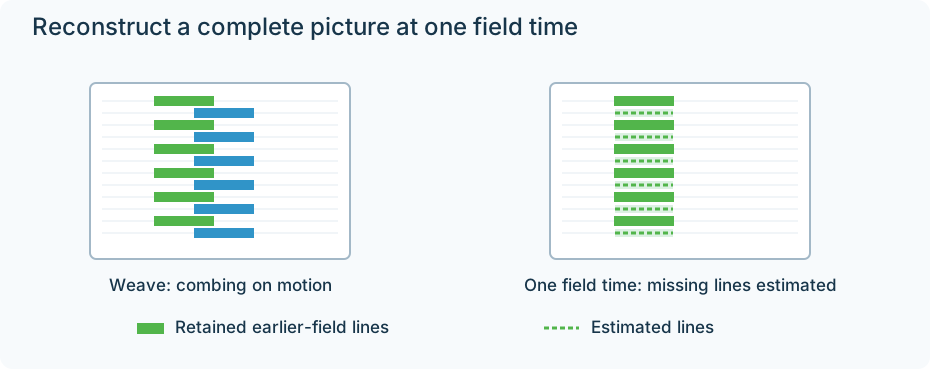
Original reduced-line schematic. It shows the principle of selecting one field's time and estimating its missing rows, rather than measured output from a named filter.
Choose the time of the output picture
Take a top-first 50-field/s recording:
- The top field describes the scene at 0 ms.
- The bottom field describes it at 20 ms.
- The next top field describes it at 40 ms.
To make a complete progressive picture at 0 ms, the top-field rows are observations from the correct time. The bottom-field rows are later observations. If an object moved during those 20 ms, directly inserting its later rows puts two positions into one picture.
A deinterlacer therefore needs more than the frame's height. It needs the field times, their order, and a rule for reconstructing the absent rows at the selected time.
The simplest reconstruction: estimate between known rows
Suppose one column in the top field contains these three brightness values at 0 ms:
| Row | Known value at 0 ms | Simple complete-picture estimate |
|---|---|---|
| 0 | 10 | 10 |
| 1 | Missing | 20 |
| 2 | 30 | 30 |
| 3 | Missing | 50 |
| 4 | 70 | 70 |
A simple vertical interpolator estimates row 1 as (10 + 30)/2 = 20 and row 3 as (30 + 70)/2 = 50. It retains the known rows and constructs the missing ones from nearby spatial information.
These are arbitrary sample values demonstrating interior-row interpolation. They are not a named filter's output or a claim that the estimates equal the unavailable camera samples. Frame-edge handling requires an additional rule.
This basic “bob” idea can produce one complete picture for each field time. It avoids weaving a later moving edge into the earlier picture. However, fine vertical patterns have been observed only on alternating rows, so their absent samples must be inferred. Thin horizontal details can soften or shimmer.
A more sophisticated spatial method can interpolate along a diagonal edge instead of only between the values immediately above and below. Following an edge's direction can keep it sharper, provided the direction estimate is sound.
Use the other field where time does not matter
For a stationary area, both fields describe the same scene. Weaving their existing rows retains more direct line information than reconstructing half the rows from one field.
The result changes with movement. Suppose the bottom field at 20 ms gives values 80 and 90 in rows 1 and 3 because a bright object has crossed the column. Weaving them into the 0 ms top field gives 10, 80, 30, 90, 70. The added rows are real observations, but of a later scene.
A moving outline can then alternate between its old and new positions on successive rows, producing combing. This is a time mismatch, not necessarily damage in the compressed file.
Blending tries a different compromise by combining information from both times. It can reduce the stark row alternation, but a moving object may leave two partially visible outlines. The picture has integrated two scene states rather than reconstructed one sharply.
Motion adaptation combines decisions within a picture
A motion-adaptive approach asks where temporal information agrees and where it changes. It can use neighboring fields or frames to compare the relevant regions.
In an area judged stationary, it can retain existing rows from both fields. In an area judged moving, it reconstructs the missing rows using spatial information and carefully selected temporal evidence. One frame can therefore contain different reconstruction decisions for its background and its moving foreground.
Detection matters because a change in sample values can come from motion, noise, lighting, or a scene cut. Repeated textures can also make matches ambiguous. A wrong stationary decision leaves combing; a wrong moving decision can unnecessarily soften a static pattern. Switching decisions around an uncertain boundary can create flicker.
FFmpeg's bwdif is documented as motion-adaptive, based on yadif with additional interpolation methods. These names identify particular implementations. The principles explain their task without assuming that every Emby server or client uses that implementation.
Preserve the field cadence
At 50 fields/s, the source has 50 native motion times. One-output-per-field reconstruction can make:
| Output time | Field providing the known rows |
|---|---|
| 0 ms | Top at 0 ms |
| 20 ms | Bottom at 20 ms |
| 40 ms | Top at 40 ms |
| 60 ms | Bottom at 60 ms |
The result is 50p, with complete estimated pictures 20 ms apart.
One-output-per-pair processing instead makes 25p, with pictures 40 ms apart. For example, retaining the earlier time in each pair keeps 0, 40, 80 ms and omits the intervening field times. Another algorithm may blend or otherwise combine them, but it still supplies fewer distinct output moments.
Both outputs can have 1080 rows and the same programme duration. The 50p representation retains the source's more frequent motion sampling. The corresponding fractional-rate pair is approximately 59.94p versus 29.97p.
Establish what the fields actually contain
The reconstruction choice begins with the source:
Native interlaced movement: each field has a new camera moment. Reconstruct complete pictures while retaining the desired field cadence.
Progressive segmented frame: both segments belong to one captured progressive frame. Pairing the correct segments recovers it; treating them as different moving moments introduces unnecessary estimation.
Telecined film: fields repeat parts of a progressive film sequence. Field matching and cadence recovery can reconstruct the film pictures from existing rows and remove their repeated presentations.
A recording can contain more than one of these structures, especially around edits and graphics. Its scan flag describes part of the format, while moving picture content reveals the capture relationship.
In an Emby playback route, reconstruction may happen in the client or during server video conversion. To understand the resulting motion, compare the source fields with the delivered progressive rate and a moving passage.
A filter can need a later field before it finishes an earlier picture, adding processing latency. The output timestamps still describe the original programme moments. Correctly scheduled audio and reconstructed pictures remain aligned even though processing took time to produce them.